Tom Goddard
January 3, 2014
James Fraser asked about how to make a difference map coloring in Chimera similar to those shown in journal article:
Picosecond time-resolved X-ray crystallography: probing protein function in real time.
Friedrich Schottea, Jayashree Somanb, John S. Olsonb, Michael Wulffc, Philip A. Anfinruda
Journal of Structural Biology, Volume 147, Issue 3, September 2004, Pages 235–246
for example, figure 6 from that article
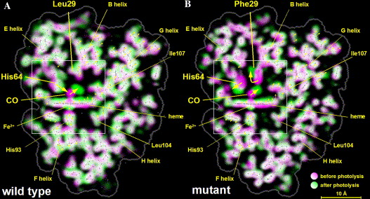
This is a difference map display where one map is green and the other is magenta. Where both maps agree the colors blend to white. It appears to be a volumetric style of rendering. Chimera is not able to blend colors in volumetric renderings of 2 maps. (This feature was in pre-2007 versions of Chimera but was removed because it was seldom used and made the code complicated and hard to had new features). I wrote a Python script do try blending the "solid" style volumetric renderings and it looks horrible in part because the grid spacing of the map is too coarse.
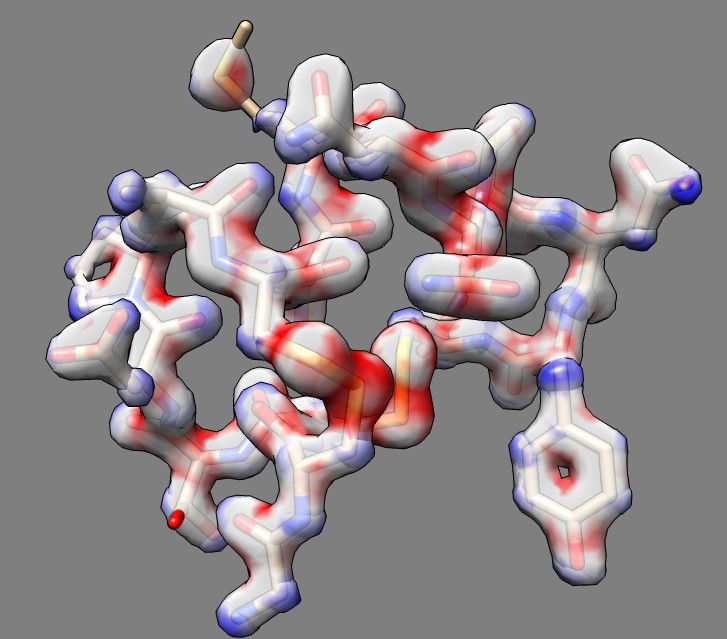
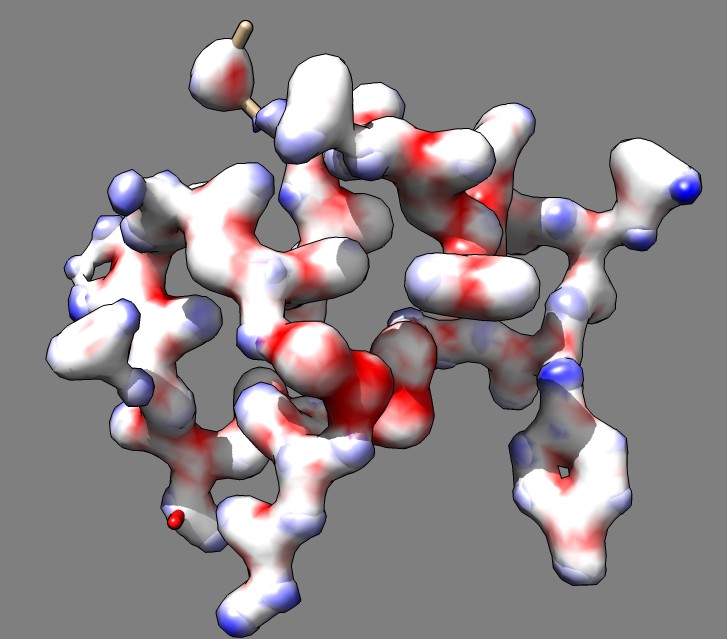
Here is an approach that uses surfaces instead of solid style rendering that I think produces a better result. Part of the aim was to be able to superimpose the molecular model on the transparent color-coded x-ray difference map. Simply subtracting the two maps and showing a contour surface is not ideal because the areas where the maps agree are not shown. The rendering we want shows the area where the maps agree, and the areas where one or the other map is larger using 3 colors. To achieve this we can show both maps with transparency and color both maps using the difference map, for instance with red where map 1 is larger, white where the maps agree, and blue where map 2 is larger. (The journal article used green and magenta because those blend together to form white, but the surface method is not restricted to complementary colors).
|
|
|
| Opacity 0.7 | Fully opaqaue. |
Here are Chimera commands to do this. As an example we will use a small protein 1a0m, it x-ray density map from the Electron Density Server, and a Gaussian smoothed copy of the original density as the second map. The command that colors the surfaces of maps #1 and #2 using difference map #3 is
scolor #1,2 volume #3 cmap -1.0,1,0,0,0.7:-0.5,1,1,1,0.7:0,1,1,1,0.7:0.5,0,0,1,0.7
The color map values (cmap argument) are density, red, green, blue, opacity separated by colons. Red, green, blue and opacity values range from 0 to 1. In this example opacity 0.7 was used and colors and density values -1.0 (red), -0.5 (white), 0 (white), 0.5 (blue) were used. The full set of commands to open the data, make the difference map and do the coloring are given below. All of these command can instead be done with menus and dialogs but the steps are harder to describe in words.
# Open PDB, show chain A atoms, hide ribbon, delete waters
open 1a0m
display :.A
~ribbon
delete :HOH

# Open x-ray map, make smoothed copy, make difference map, set transparent colors and threshold levels
open edsID:1a0m
vop gaussian #1 sDev 0.5
vop subtract #1 #2 minRMS true
volume #1 show color 1,0,0,.5 level 1
volume #2 show color 0,0,1,.5 level 0.5
volume #3 hide

# Show only the density within 2 Angstroms of the atoms.
sop zone #1,2 #0:.A 2

# Change background color and show silhouette edges
set bg dimgray
set silhouette

# Color two maps based on the difference map value at the surface points
# The colormap (cmap) argument lists density,red,green,blue,opacity values separated by colons.
# Red, green, blue and opacity values are in the range 0 to 1.  Example uses opacity 0.7.
scolor #1,2 volume #3 cmap -1,1,0,0,0.7:-0.5,1,1,1,0.7:0,1,1,1,0.7:0.5,0,0,1,0.7
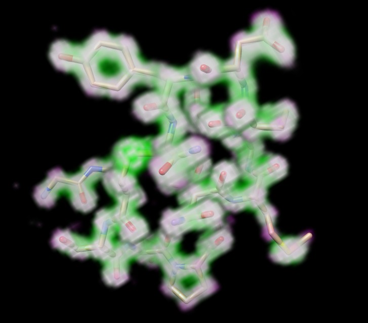
Here is an image of solid style rendering done with blending the two maps using magenta and green colors done with a Python script. Looks horrible. The grid artifacts could be reduced using maps with finer grid spacing. But the lack of 3-dimensional appearance is caused by not having lighting cues in solid style rendering and that cannot easily be improved.