The purpose of this exercise is to get familiar with Chimera features for display of density maps and models of large molecular assemblies.
This tutorial is based on Chimera version 1.2105 (March 2005). Some features described may have changed in more recent Chimera versions.
This tutorial uses a PDB file and a density map of Semliki Forest virus that you can download from this web site (1DYL.pdb, emd_1015.map) or from the PDB and Macromolecular Structure Database web sites (1DYL.pdb, emd_1015.map).
Density map topics:
Atomic model topics:
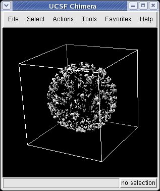
Use the Chimera File / Open dialog to open emd_1015.map. In the File Open dialog you should change the File Type to All (guess type). Initially it is set to only show Protein Data Bank files (*.pdb).
The Volume Viewer dialog will appear. Press the Show button at the bottom of that dialog to see the map. Small density maps (< 1 million voxels) are displayed immediately when you open them, but larger maps are not displayed until you press Show so that you can first choose a subregion of the map if desired.
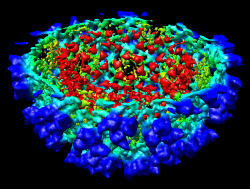
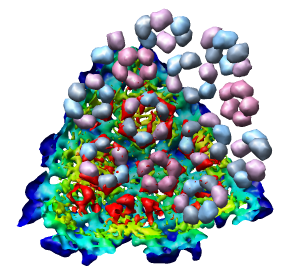
This 9 angstrom resolution density map is a single particle reconstruction from electron cryo-microscopy. The virus surface consists of glycoproteins embedded in a lipid envelope. Inside that layer is a protein shell of 240 copies of the nucleocapsid protein, and inside that is packed the single-stranded viral RNA genome. The lipid and viral RNA are not arranged with icosahedral symmetry and are not visible in this density map. This density map emd_1015.map and others are available from the EM database.
Dragging the mouse in the graphics window lets you rotate, translate, and zoom in on the map.
On a Mac with a one button mouse, hold down the Option key to get middle mouse button behaviour, or the Command key to get right mouse button behaviour.
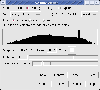
Controls for display of volume data (ie density maps) are in the Volume Viewer dialog that was displayed when you opened the file. If you close this dialog it can be shown again with menu entry Tools / Volumes / Volume Viewer.
The histogram in the center shows the distribution of data values in the density map. The range of data values (-24916 to 25619) is shown below the histogram. The white vertical bar on the histogram shows the contouring threshold. Drag this bar with the mouse to change the contour level. The numeric value of the contour level is shown below the histogram in the entry field. Contour levels can be typed in instead of being set with the mouse.
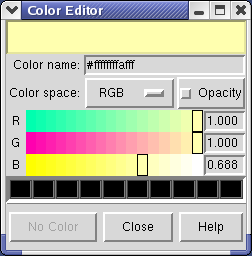
Clicking on the white square with the wide raised border below the histogram shows a Color Editor dialog. The square button, called a Color Well, is used in many Chimera dialogs to choose colors and shows the current color in the center. Change the density map color by clicking on the color bars in the Color Editor dialog. You can close the dialog when you are done.
Above the histogram is a radio button where you can choose mesh display style. This shows the surface as a mesh made up of triangles. You may need to zoom in to see the small triangles.
Near the top of the dialog the data size, 301 by 301 by 301, is shown. The Step menu allows you to subsample the data. For this large map, the initial step is 4 4 4 which means to use every fourth density value along each of the 3 axes. The 1 1 1 step setting shows full resolution data -- but don't try that highest resolution setting now because it will be very slow to compute the surface and render it (~1 minute). Later when we restrict the display to a smaller piece of the map we will use higher resolution.
The outline box shows the bounds of the data set. You can hide the outline box by clicking the Options checkbutton on the right side of the top line of the Volume Viewer dialog. This displays a panel of options and the first one Show outline box... can be switched off. Clicking the Options checkbutton again hides the long panel of options.

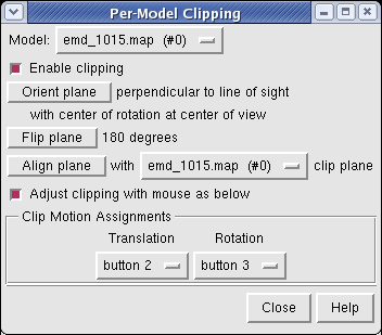
The Tools / Graphics / Per-Model Clipping menu entry lets you slice through surfaces (and atomic models). Turn on the Enable clipping switch in the dialog that is shown. Then rotate the density map to see the cut.
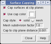
The cut surface is visually confusing because you see inside of the surface. Use the Tools / Graphics / Surface Capping menu entry and switch on Cap surfaces at clip planes. This will cap the hole where the surface was cut. To make the cap a different color than the surface click the Use cap color... switch on the Surface Capping dialog.
To move the cut plane, also called the clipping plane, switch on the Adjust clipping with mouse... switch in the Per-Model Clipping dialog. Then drag the clip plane with the middle mouse button or rotate it with the right mouse button.
Turn off the Adjust clipping with mouse... switch to restore the mouse buttons their normal behaviour of translating models and zooming.
|
|
|
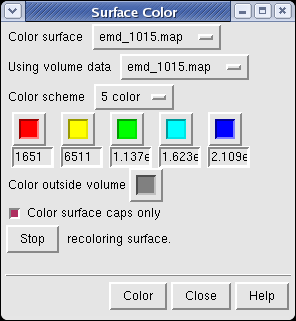
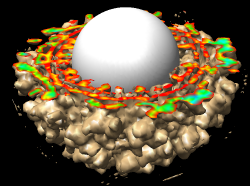
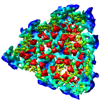
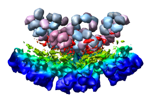
The density map values vary across the clipped capped surface. The variation can be shown by coloring the cap using Tools / Volumes / Surface Color. Change the Color scheme in the Surface Color dialog to be 5 color. (The 3 color color scheme is intended for display of electrostatic potentials.) To only color the cap switch on Color surface caps only. Then press the Color button at the bottom of the dialog. When you move the clip plane, the coloring will be automatically updated.
It is useful to color the density according to distance from the center of the virus in order to see the layers. To do this use menu entry File / Open and open radius.nc. This is another volume data set where each grid point value is the distance to the center of the virus. The Volume Viewer dialog will now show a histogram of the radius map, and moving the threshold vertical bar on the histogram will show spheres of different radii in the graphics window.
| 
| 
|
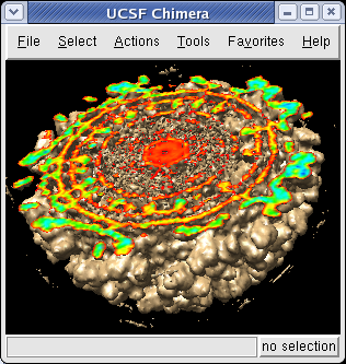
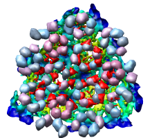
Press the Unshow button at the bottom of the Volume Viewer dialog. We do not need to see the radius map isosurface. In the Surface Color dialog choose radius.nc from the Using volume data... menu on the second line, turn off Color surface caps only and press the Color button at the bottom of the dialog. Now the coloring of the virus surface is done using the values of the radius map.
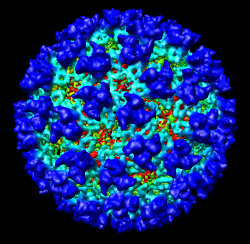
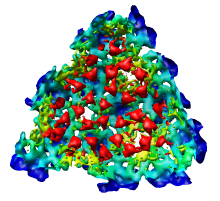
To see the layers of the virus better, change the default radii for the red, yellow, green, light blue, and dark blue colors given in the Surface Color dialog under the color buttons to 200, 225, 250, 275, and 300 respectively and press the Color button at the bottom of the dialog to use these new values. These radius values are in angstroms. The virus has a radius of about 350 angstroms.
Adjusting the virus map threshold level to approximately 8000 in the Volume Viewer dialog shows the nucleocapsid proteins as red blobs. To adjust the virus map select emd_1015.map using the the Data menu on the second line of the Volume Viewer dialog. That menu allows you to switch between the virus map and radius map that you have opened so far.
Opening a special radius map file to color radially is cumbersome and in a future Chimera release (not yet in 1.2105, March 2005) we will provide radial coloring and other geometric colorings without having to load any special volume file.
|
|
We'll now show just one octant of the semliki density map. Turn off the Enable clipping switch in the Per-Model Clipping dialog, and turn off the Cap surfaces at clip planes switch in the Surface Capping dialog and close those dialogs.
Click the Region checkbutton and the Options checkbutton on the top line of the Volume Viewer dialog, and turn on the Show bounds and step in region panel switch that appears as the eighth line in the list of options. You should then see a line in the volume dialog just above the long list of options that looks like:
Region min max step x [0 300 4] y [0 300 4] z [0 300 4]
The 0 and 300 values are the minimum and maximum voxel indices and the 4 values are the step sizes for the x, y and z axes. Type in new values
Region min max step x [150 300 2] y [0 150 2] z [150 300 2]
and press the Enter key on the keyboard in any one of those entry fields to show one octant of the virus map.
Note that we changed the step size from 4 to 2 because the computer can handle this smaller piece of the density map at higher resolution.
You can uncheck the Options button at the top of the volume dialog to remove the options panel from the dialog.
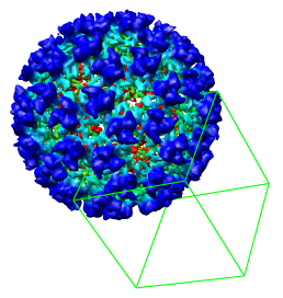
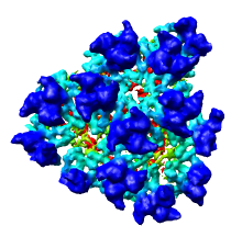
As an alternative to typing the numeric bounds of the density map subregion you can interactively choose the octant using the mouse. To redisplay the full density map press the Back button.
Switch on Select subregions using button 2 near the bottom of the volume dialog. Press the Orient button on the Volume Viewer dialog, one row from the bottom to return the density map to the original orientation it had when you opened it. Then drag with mouse button 2 from the center of the virus particle toward the lower right corner of the graphics window. This will create a 3 dimensional green outline box. By rotating the model and and then dragging with mouse button 2 over any of the six faces of the box you can adjust the outline box size.
After enclosing just one octant of the virus particle press the Crop button on the Volume Viewer dialog to show just the data in that green box. If you did not get one octant, press the Back button to return to viewing the entire density map. When you have displayed just one octant of the map, turn off the Select subregions using button 2 switch on the volume dialog so that mouse button 2 will return to its normal function of translating the models.
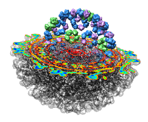
We now look at an atomic model of the nucleocapsid protein determined by x-ray crystallography that has been fit into the density map.
Use File / Open to open Protein Data Bank model 1DYL.pdb. It is in the same directory as the density map. The purple wire depiction of the atomic model will be shown.
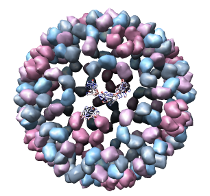
Only 1/60th of the nucleocapsid is shown. Use menu entry Tools / Multiscale / Multiscale Models and press the Make models button at the bottom of the Multiscale dialog to show the full icosahedral capsid. This is using 60 matrices specified in the PDB file header to replicate the atomic model. Each of the 240 proteins is now displayed as a low resolution surface derived from the atomic model.
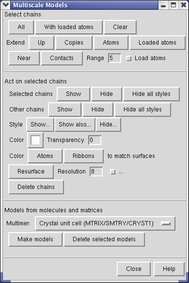
Select the half of the capsid not contacting the piece of the density map by dragging out a box with Ctrl mouse button 1. Then press the Hide button on the line of the Multiscale dialog that says Selected chains.
The Multiscale dialog is divided into 3 sections by horizontal lines. The top section has buttons for selecting parts of the multimeric atomic model. The middle section is acting on the selection (hiding, showing, coloring, changing display styles). The bottom section is for creating multimeric models.
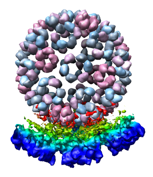
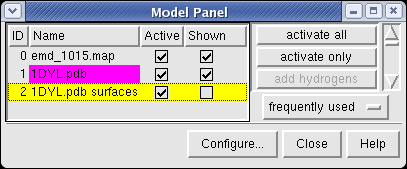
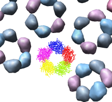
Looking at the agreement between the atomic capsid model and the density map shows that they do not align. Look at the rings of 5 proteins (5 pink blobs) and the rings of 6 proteins (6 blue and pink blobs) in both the atomic model, and the density map (red blobs). Hide the atomic model by unchecking the button in the Shown column of the Model Panel dialog (menu Favorites / Model Panel) next to 1DYL.pdb surfaces to see just the density map.
There is a mismatch in coordinate systems being used by the PDB model and density map. This is an error in the deposited data, which is unfortunately rather common.
We will now make an approximate alignment by hand.
The atomic model and density map appear to center the virus at the same point. So we will try to rotate the atomic model about the center of the virus to align it with the density. Notice that rotating the scene with the mouse does not rotate about the virus particle center. The normal rotation center is the center of a box containing the displayed models.
To change the center of rotation hide the density map by turning off its Model Panel shown button and show the 1DYL.pdb surfaces model. Press the All button at the top of the Multiscale dialog, and the Show button on the Selected chains line of that dialog. Now just the atomic model of the full capsid is shown and rotation with the mouse happens about its center. Use menu entry Tools / Viewing Parameters / Rotation and set the center of rotation method in the Viewing dialog that appears to fixed. Now reshow the density map and reselect half of the atomic capsid and hide it as you did earlier.
To move the atomic model without moving the density map switch off the button in the Active column of the Model Panel dialog next to emd_1015.map. Now try to rotate the atomic model with the mouse to align it with the density. A good strategy is to move the pink ring of 5 proteins to coincide with the ring of 5 red density blobs. Then rotate by dragging the mouse near the edge of the graphics window to rotate about the z-axis (perpendicular to the screen) to make the rings of 6 proteins match. Iterate a few times. It's not easy. When you get a satisfactory alignment turn back on the Active switch for the density map in the Model Panel dialog so both models move together.
If you accidentally translate the atomic model relative to the density map (using mouse button 2) the centers will no longer coincide. To correct this use menu entry Tools / Utilities / Undo Move to get back to a point before you did the accidental translation.
Now we'll look at atomic details of the nucleocapsid. Hide the density map by clicking off the button in the Shown column of the Model Panel next to emd_1015.map.
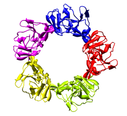
We'll look in atomic detail and a ring of 5 pink proteins. These lie at the 5-fold symmetry axes of the icosahedral virus particle. Select 5 of the pink proteins that form a ring. Use ctrl left mouse button to select one of them and shift ctrl left mouse button to add each of the remaining 4 to the selection. On the Multiscale dialog press the Show... button on the Style line (near the middle) and choose Wire from the menu that pops up.
Press the Hide button on the Other chains line of the Multiscale dialog. This hides the unselected proteins. (Technically "other chains" refers to ones that are not selected but are within a model that has some chains selected.) This hides all but the 5 proteins for which we are showing all atoms in wire style.
You will notice that rotation is still happening about the center of the virus particle. That is inconvenient now. Use Tools / Viewing Parameters / Rotation and set the center of rotation method back to center of models. Now mouse rotations will occur about the center of the 5 protein ring being displayed.
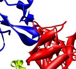
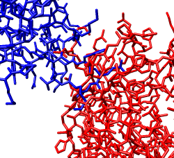
Zoom in close and look at the contacts between neighboring proteins. Notice there are contact clashes. The interfaces between neighboring proteins are not physically reasonable. Use the Show... button on the Style line of the Multiscale dialog and try different representations (sphere, stick, ribbon).
We can color the atomic models according to the density map values. Use Model Panel to select the original copy of 1DYL that we opened, model id 1. You will see additonal copies that were created to represent the pentamer ring we just looked at. Click on the first 1DYL.pdb line in the Model Panel and then press the Select button in the right hand column. Now press the Multiscale dialog Show... button on the Style line and select Ribbon from the popup menu, and press the Hide all styles button on the Other chains line. This shows 4 protein monomers (the asymmetric unit) as ribbons. You may need to zoom out to find them (right mouse button).
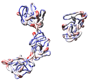
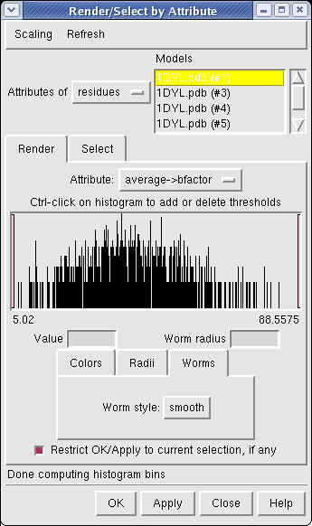
Now use menu entry Tools / Graphics / Render by Attribute. We are going to use the fact that the 1DYL file from the Protein Data Bank has the density of the electron microscope map at each atom position encoded in the B-factor column of the ATOM lines. This is not related to a crystallographic b-factor, and is just a creative misuse of the PDB file format.
In the Render by Attribute dialog choose Attributes of residues and below that choose Attribute average b-factor, then press Apply at the bottom of the dialog. Now the ribbons are colored blue to indicate high density and red to indicate low density. Click on the Worms tab near the bottom of the Render by Attribute dialog and press Apply again to make the thickness of the ribbon also correspond to the density. Fat areas are low density indicating regions where the atomic model does not lie in high density regions of the density map.
The "b-factor" value is a scaled representation of the density where 100 corresponds to minimum density and 1 the maximum density. The histogram in the Render by Attribute dialog shows the distribution of these values.
Rotating models is much slower when something is selected because it requires alot of computation to compute the green selection outline. Unselect everything using ctrl left mouse button on the background to get faster rotation.
Looking at the protein-protein interfaces you'll see that the contact clash for one pair of proteins is blue (in high density) and for another pair is red (in a low density region).
With a ctrl left mouse drag select all 4 protein worms and press Show on the Other chains line of the Multiscale dialog to see the locations of the protein monomers in the full nucleocapsid. You may need to adjust the front clipping plane with the side view dialog (menu entry Favorites / Side View) so the full particle is not clipped.
The Tools section of the Chimera User's Guide contains more information on the features covered in this tutorial.
The Chimera web site is at http://www.cgl.ucsf.edu/chimera