Electrostatic potential.

Crystal difference maps.

Solvent occupancy.
July 15, 2008
These 6 volume exercises are independent of one another and can be done in any order. You can try them with your own data or the suggested data sets.
Download the data sets for exercises as needed.
More examples of Chimera volume features can be found in the Guide to Volume Data Display.
|
Electrostatic potential. |
Crystal difference maps. |
Solvent occupancy. |

Morphing between maps. | 
Erasing part of a map. | 
Tracing surfaces. |
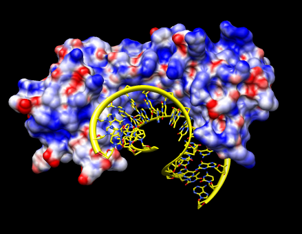
We'll look at the electrostatic potential of a DNA binding protein 1qna. The DNA phosphate backbone is negatively charged. Interaction with positive charge on a protein can contribute to binding.
The electrostatic potential is computed on a 3-dimensional grid by programs such as APBS, DelPhi, and UHBD. Chimera does not compute the potential. We'll use a potential file that has already been computed using APBS.
Open 1qnaA.pdb and create a molecular surfaces, Actions / Surface / Show. Open potential volume data 1qnaA.dx which will show the Surface Color dialog. Press the Color button on the Surface Color dialog.
Blue shows positive potential, red negative, with transparent white being neutral (zero potential energy). Try changing the potential values to -20 and 20 for red and blue and press Color. The units of these potential energy values are kT/e, where temperature T = 298.15 was set in the APBS potential calculation. Try changing the transparent white color to solid white by clicking on the color well, adjusting the color opacity (A slider), and pressing the Color button.

The "A" at the end of the file names refers to chain A of 1qna which is the protein. The 1qna entry also contains the DNA, but we are interested in the electrostatic potential for only the protein. Open 1qnaCD.pdb to show the DNA. Select a DNA atom and press the "up arrow" keyboard key 3 times to select the entire DNA and show round ribbons, sticks, and color by element (Actions menu entries Ribbons / show, Ribbons / round, Atoms / stick, Color / by-element).
If you didn't want to go to the trouble of computing electrostatic potential with solvent screening using external software that solves the Poisson-Boltzmann equation, you can get a crude approximation by selecting residues that normally (pH 7) have positive charge and coloring them blue, then selecting residues types with negative charge and coloring them red. Use menus Select / Residue / Amino Acid Category and Actions / Color.
To use APBS you first need to assign charges to each atom. This can be done with the pdb2pqr program or the pdb2pqr web service. Using the web service you submit your PDB flie on a web page, click the "Create an APBS input file" option, and get back a "*.pqr" file that is the PDB with charges added, and a "*.in" file that sets APBS parameters. With APBS installed on your computer you run apbs on the "*.in" file from a terminal. After some minutes it produces the pot.dx potential file.
Crystallographic maps don't exactly agree with the PDB model that is derived from them. This can be because parts of a protein are flexible or assume multiple conformations or the model does not include all atoms present in the crystal. More information can be gleaned by looking at the crystallographic map, especially at critical places in proteins structures such as binding sites.
We'll look at a structure of an antibody fragment and an HIV protease peptide, 1svz.pdb, the crystallographic map the PDB file was derived from 1svz.omap, and a "difference map" 1svz_diff.omap representing errors between the PDB model and the map. The two maps were obtained from the Uppsala Electron Density Server and can be fetched directly by Chimera using the PDB ID (File / Fetch by ID) if they weren't provided with this tutorial. Open these 3 files.

There are two copies of the antibody and bound hiv peptide. We'll look in detail near bound peptide chain D. Select chain D (Select / Chains / D). Then show maps in a box around chain D using volume dialog Features / Atom Box. Set the padding value to 4 Angstroms and press the Box button. That limits the volume display for just one of the maps, the that is highlighted in the volume dialog. Click on the name of the other map in the volume dialog and press the Box button to display the same small subregion for it.
Hide the parts of the PDB model except near chain D. Here's one way to do that. Hide the ribbons (Actions / Ribbon / hide). Select chain D (Select / Chain / D) and extend the selection to a 4 Angstrom zone around it (Select / Zone..., check "Select all atoms of any residue in zone", press OK), invert the selection (Select / Invert), and hide those atoms (Actions / Atoms / hide). Color chain D yellow so the peptide is easy to distinguish from the antibody residues.
Hide the difference map (click the "eye" icon on the line above its histogram in the volume dialog), and adjust the contour level of the other map so the residue shapes can be seen (level ~0.2), and change to mesh display using the button in the volume dialog.
The difference map shows discrepancies between the PDB model and the crystal map. Redisplay the difference map (eye icon above histogram), change it's color to red, and adjust its contour level so there are not too many red blobs. These are areas where there is extra density in the experimental crystal map that is not accounted for by the PDB model. To reduce the confusion of lines you can change the crystal map to "surface" style and make it transparent so the model appears through it.
Negative values of the difference map indicate regions where the experimental crystal data shows too little density for what is expected from the PDB model. To show those regions add a second contour level to the difference map by holding the "ctrl" key and clicking on the histogram. With a negative contour level a solid box appears in the graphics window because almost all the difference map data lies above that level. Fix this problem using volume dialog Features / Surface and Mesh Options, and turning off "Cap high values at box faces" near the bottom of the list of options. Color the negative contour surface blue using the volume dialog color button.
The color zone tool (volume dialog Tools menu) can be used with chain D selected to color the crystal map near the ligand yellow.
Another way to see what the difference map says about discrepancies in the PDB model is to animate the map to show missing and extra density. This can be done with the Morph Map tool (volume dialog Tools menu) using maps 1svz.omap and 1svz_diff.omap, enabling "Add to first map..." and using movie start = -1 (predicted density from model), end = 0 (experimental density). Quicktime movie. An explanation of the morph map tool is given in the "Morph between Maps" exercise.
We'll make volume data sets showing where water is localized around part of a protein in a molecular dynamics simulation. The water molecules move around but Chimera can count how often a water is found in each cell of a grid placed around the protein. We'll use a molecular dynamics simulation of a beta hairpin from protein G provided by John Chodera.
Start the MD Movie tool, Tools / MD+Ensemble Analysis / MD Movie. Choose trajectory format Amber, Prmtop file hairpin_prmtop.gz, and Trajectory hairpin.trj.gz, and press OK. Color by element (Actions / Color / by element). To see the hairpin better through all the surrounding water, select it (Select / Chain / (no id)). Press the play button (right pointing triangle) in the movie dialog to see the trajectory.
We have to hold the hairpin steady for the water occupancy grid to accumulate useful information about where waters localize around the hairpin. Select the hairpin (no id). We would like to use Actions / Hold Selection Steady. But three sodium ions are also selected and they jump across boundaries of the periodic octahedral box of water. For simplicity, delete them with command "del @Na+" (menu Favorites / Command Line). Then use Hold Selection Steady. When the trajectory is played, the hairpin will no longer drift in the water.
To compute the water occupancy maps, select the water (Select / Chain / water) and use movie dialog Analysis / Calculate Occupancy... and press OK. Hide the water to see the maps (Actions / Atoms / hide). One map shows where the water hydrogens are most frequently found, and the other where the oxygens sit. Raise contour levels to hide noise and color the oxygen and hydrogen maps to make them stand out from the atomic model.
Notice about 5 locations show oxygen and hydrogen blobs that suggest the water has a preferred orientation possibly due to transient hydrogen bonds with the hairpin. A movie (quicktime, 40 Mb) showing the hydrogen bonds to nearby waters throughout the trajectory supports this idea.
To see the differences between two maps representing for example different conformations of a molecular assembly you can use the Morph Map tools. This shows one map smoothly turn into another map. The method for producing the intermediate maps is to interpolate the maps at each grid point and compute the contour surface for the interpolated map. The maps must have the same size and be aligned.
We'll look at two electron microscopy maps of human RNA polymerase II, a twelve protein complex that transcribes chromosomal DNA to RNA. Two conformations were observed producing rnapii_1.map and rnapii_2.map. Open these maps.
To set a reasonable contour level we'll use that the molecular weight of this complex is about 450 kDa. Globular proteins usually occupy about 1.21 Å3 per Dalton (Harpaz 1994). So choose a contour level to make the surface enclose about 544,000 Å3. Use volume dialog Tools / Measure Volume and Area and interactively adjust the contour level to produce approximately the desired volume.
Use volume dialog Tools / Morph Map and press the Play button to see the interpolated maps. The contour level stays fixed when the interpolated maps are shown and because the normalization of the two maps is a bit different the map appears to shrink when going from rnapii_1.map to rnapii_2.map. To compensate for this the contour level can be automatically adjusted to preserve volume. Turn on "Adjust threshold for constant volume" and press Play.

| 
| 
| 
| 
|
The calculation in Chimera can be slow. Increasing the step size of the interpolated map in volume viewer can speed it up. To get a smooth variation it helps to record a movie using the Record button on the morph map dialog. You may wish to change the morph dialog step size from 0.1 to 0.02 so that 50 frames are recorded instead of 10. Movie playback speed is 25 frames per second. The morph is recorded forward than backward so that it ends where it started so that looped playback has no abrupt transitions. (There's a "loop" option in QuickTime player 7.5 under the View menu.) Quicktime movie (1 Mb).
It is sometimes useful to erase part of map to extract the density for just one object of interest. Will use this to extract the conical HIV virus core that contains he RNA from electron microscope tomography data.
Open the HIV virus particle map hiv.mrc and start the volume eraser tool from the volume dialog Tools menu. A transparent pink ball will be shown that can be moved around with the middle mouse button. Holding the shift key allows moving the ball into and out of the screen. Pressing the Erase button erases the volume data values within the sphere. A new copy of the partially erased volume data is made and it can be saved to a separate file.
To get at the conical core inside this virus you can place the pink sphere inside the capsid. Use a sphere radius of about 550 Angstroms set with the slider in the eraser dialog. To erase outside you type a keyboard shortcut which is two keys "eo". You have to turn on keyboard shortcuts using menu entry Tools / General Controls / Keyboard Shortcuts and click "Enable keyboard shortcuts". Then type "eo" in the main grahics window. The density outside the sphere will be erased.
|
| 
|

| 
|
The conical core is surrounded by "debris" that is thought to be left-over nucleocapsid protein that coats the core. Using a small pink sphere this debris can be erased. There is no undo when erasing so periodic saving of the erased map is advised.

|
|
We'll hand trace a surface in order to extract the conical core particle of HIV virus that contains the RNA genome. The surface is created by drawing loops with the mouse in several planes slicing through the virus. Then the loops are joined to form a surface. The density within the surface can then be put in a separate map using the "mask" command.
Open map hiv.mrc. This is one particle from EMDB entry 1155, electron tomography, Gaussion smoothed with 50 Angstrom standard deviation and resampled so that the conical core has its axis approximately parallel to z. Show a single plane (volume menu Features / Planes, press One button, set axis to Z). Adjust histogram nodes to contrast core from background.
Use volume dialog Tools / Volume Tracer to draw loops on a data plane. Use tracer Features / Mouse Mode Options and turn off "Place markers on spots" and turn on "Place markers on data planes" and "Place markers while dragging", and set "Dragging marker spacing" to 3. Now hold down the middle mouse button and draw a loop on the data plane. When you get near the marker you started with the loop will automatically close. To change the loop color select the markers (drag box with ctrl left mouse button) and use the marker color button in the tracer dialog. Trace loops in several planes. Delete unwanted markers or loops by selecting them and using tracer menu Actions / Delete markers.
To create a surface use tracer menu Features / Surfaces. To make a surface from all the loops make sure all of them (or none of them) are selected. Press the surface Create button.
To create a separate map containing just the density within your surface, select the surface, and use command "mask #0 sel" (Favorites / Command Line). Here #0 is the id number of the original hiv map. Hide the surfaces with Actions / Surface / hide. Change the new map to surface display style and color it using the volume dialog color button. Redisplay the original map so the core can be seen within the original map.

| 
| 
|