Command: volume

Usage:
volume  model-spec   options

The volume command controls the display of density maps and other volume data, i.e., values associated with points on a 3D grid. The model-spec can be a specific model number or range of model numbers (preceded by #), or the word all to indicate all volume models. The model-spec can be omitted for certain options that can or must apply globally, namely pickable and several of the sampling and size options.

The corresponding graphical interface, Volume Viewer, allows adjusting contour levels and some of the other settings interactively. Contour levels can also be changed interactively with the mouse mode for contour level or windowing .

Volume data can be opened with the command open (which automatically starts Volume Viewer) and saved to a file with save. By default, a data set will be displayed automatically if it does not exceed a certain size, and the initial display may be as an isosurface or as a single plane (details...). Many settings for newly opened data, including the size limits controlling these behaviors, can be customized with the volume defaultvalues command.

The initial contour level of an isosurface is set to enclose 1% of grid points, except for maps opened by EMDB fetch, which will be shown at the depositor-recommended contour level, if any. For single-plane display, the middle plane along Z is shown initially with a linear ramp in grayscale from the 10th (black) to 99th (white) percentile of values.

Data set statistics, isosurface-enclosed volumes, and map-map correlation values can be reported with measure. See also: show, color, transparency, vseries, molmap, fitmap, resfit, surface operations, sym, smoothlines, segmentation, Map icons, Medical Image icons, measurements, ChimeraX DICOM Reference

volume #1 style mesh level 0.8 color red level 1.2 color 0,50,80
volume #2 level 10,0 level 100,1 level 400,1 color hot pink style image
vol all hide
vol channels #2-8
vol settings #1
vol defaultvalues limitVoxelCount false saveSettings true
vol default reset true

The command volume channels (followed by a model-spec, as in the example above) groups the specified volume models into a single multichannel data set, where changing the display style, step size, crop boundaries, or display plane of one channel in the Volume Viewer interface or with the mouse changes it for all of the channels in the group. The channels are grouped as submodels of a single higher-level model. Settings for the individual channels can still be changed independently with other options of the volume command.

The command volume settings (optionally followed by a model-spec) reports volume model properties and display settings in the Log. See also: info

General Display Options
Sampling and Size Options
Dimension and Scale Options
Planes Options
Surface and Mesh Display Options
Image Display Options
Setting Defaults for New Maps
Volume Operations (Map Editing)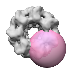

[back to top: volume]

General Display Options     (Usage: volume  model-spec  options)

• show
Display the volume model.

• hide
Undisplay the volume model.

• toggle
Of the specified volume models, show those that are hidden and hide those that are shown.

• style  surface | mesh | image
Designate the style of display: the surface and mesh modes show isosurfaces (contour surfaces), while the image mode (synonym solid) refers to a cloudlike display with varying intensity and opacity.

• close  surface | image
Close submodels with display style surface (including both surface and mesh) or image.

• pickable  true | false
Whether a volume model should be selectable with the mouse (initial default true). This setting can be applied to individual models, but if the model specification is omitted, the setting is global and applies to all volume models, including those opened later within the same session.

• level  threshold-level 
Place a threshold for mapping data values to the display. Can be given multiple times in the same command for multiple contour levels on the same volume data.

• For surface and mesh displays, threshold-level is a single number, the contour level of the surface. This corresponds to horizontal placement on a histogram in the graphical interface. To adjust the threshold level automatically so that the contour encloses a specified spatial volume, see the encloseVolume and fastEncloseVolume options.
  
  
• For image displays, threshold-level consists of two numbers separated by a comma (no spaces). The first number indicates a data value and the second number indicates an intensity ranging from 0.0 to 1.0. These correspond to horizontal and vertical placement, respectively, on a histogram in the graphical interface.

Threshold levels can be adjusted interactively by dragging in the Volume Viewer histogram or by using the mouse mode for contour level or windowing in the graphics window.

• rmsLevel  threshold-level 
• sdLevel  threshold-level 
Same as level, except with threshold-level specified in units of root-mean-square (RMS) deviations from zero or standard deviations (SD) from the mean, respectively, calculated for the current display region and step size. See also: volume scale, measure mapstats

• color  color-spec 
Assign threshold color. Can be given multiple times in the same command if multiple threshold levels are also specified. To specify initial colors for maps that have not yet been opened, see the initialColors option.

• initialColors  color-list
Specify initial colors for subsequently opened maps as a list of color specifications separated by commas only. Applies to the current session only, but can be used with volume defaultvalues to customize future sessions, for example:

volume defaultvalues initialColors salmon,lime,#ff805c save true

The factory defaults are . See also: initial colors

• brightness  value 
Brightness scales the intensity of the color (default 1.0). A value greater than 1.0 may be used, but the RGB color components multiplied by the value are clamped to the range 0.0–1.0.

• transparency  value 
Transparency values range from 0.0 (fully opaque) to 1.0 (fully transparent).

• For surface and mesh displays, transparency is the fraction of light transmitted from behind the surface or a line of mesh (default 0.0). By default, these objects are dimmed as they are made more transparent (see dimTransparency.) See also:
  
  
• For image displays, this setting gives the slab thickness (as a fraction of the dataset's shortest dimension, range 0.0–1.0, default 0.5) that gives the transparency indicated by threshold height on the histogram (details...). By default, more transparent voxels are made dimmer (see dimTransparentVoxels).

• change  surface | image
The change option is only needed to change settings of a hidden display style when a volume model has both surface (surface and/or mesh) and image submodels. It applies to settings specified with level, rmsLevel, sdLevel, color, brightness, and transparency. If change is not used, the setting applies to whichever style is currently shown.

• encloseVolume  volume
Automatically set surface or mesh threshold level to enclose the specified volume in distance units cubed (e.g., ų if the grid spacing is expressed in Å). Multiple volume models can be specified in the same command to make their isosurfaces enclose the same spatial volume. The level is determined by an iterative procedure. In each iteration, the density value midway between the upper and lower bounds is tested. If the resulting enclosed volume is larger (smaller) than the target, that midpoint value becomes the new lower (upper) bound. In the first iteration, the upper and lower bounds are the maximum and minimum values in the map. Iteration stops when the actual enclosed volume differs from the target by less than 0.001 of the target or 30 iterations have been performed. The enclosed volume is computed only within the rectangular box of the current display region, but this may include parts hidden due to zoning. The fastEncloseVolume option is similar but uses a noniterative approximation. See also: vseries align, measure volume

• fastEncloseVolume  volume
Automatically set surface or mesh threshold level to enclose the specified volume in distance units cubed (e.g., ų if the grid spacing is expressed in Å). Multiple volume models can be specified in the same command to make their isosurfaces enclose the same spatial volume. The number of grid points to enclose is estimated by dividing the target volume by the volume of one grid cell, and then the level corresponding to that number of points is estimated by sorting the data values into 10,000 bins of equal width and identifying the value bin that attains (cumulatively) that number of points. The enclosed volume is computed only within the rectangular box of the current display region, but this may include parts hidden due to zoning. The encloseVolume option is similar but uses an iterative procedure with increased accuracy at the cost of increased computation time. See also: vseries align, measure volume

• showOutlineBox  true | false
Outline the bounding box of the current display region.

• outlineBoxRgb  color-spec
Assign a color to the outline box (default white). Any transparency in the color will be ignored.

• calculateSurfaces  true | false
Whether to force calculating a volume isosurface immediately rather than at the next graphics frame update. Setting this option to true in a volume command that modifies surface geometry (for example, setting the level) is needed when another command that would use the surface geometry is appended to it with a semicolon separator, which indicates no graphics frame update between the commands. See: ChimeraX command files

[back to top: volume]

Sampling and Size Options     (Usage: volume  model-spec  options)

• step  N | Nx,Ny,Nz
Step values indicate sampling density; a step of 1 means all data points are used to generate the display, while 2 means every other data point is taken along each axis. Step sizes must be integers. If a single number is supplied, it is used in all three directions; if three numbers are supplied (separated by commas but not spaces), they are used in the X, Y, and Z directions, respectively. Changing a step value will change the data size limit for automatic step adjustment (see voxelLimit). See also:

• limitVoxelCount  true | false
Automatically adjust step size so that no more than the specified voxel limit is displayed.

• voxelLimit  limit
Set the maximum number of Mvoxels to be displayed (default 1.0) when limitVoxelCount is set to true.

• showOnOpen  true | false
Automatically display a data set when it is opened if it does not exceed a specified size.

• voxelLimitForOpen  size
Set the data size limit in Mvoxels below which data should be automatically displayed when opened (default 256.0) when showOnOpen is set to true.

• showPlane  true | false
Initially display just a single plane (normal to the Z axis) of a data set if it exceeds a specified size.

• voxelLimitForPlane  size
Set the data size limit in Mvoxels above which a single plane of the data should be initially displayed (default 256.0) when showPlane is set to true.

• dataCacheSize  size
Set how much memory in Mb should be dedicated to volume data (default is half the physical memory in the computer). A cache can improve performance, since accessing cached data is faster than reading it from disk. The least recently displayed data values are purged to maintain the specified size. The data cache only accounts for approximately 1/3 to 1/2 of the memory used in viewing volume data, as additional memory is occupied by surfaces and color arrays.

[back to top: volume]

Dimension and Scale Options     (Usage: volume  model-spec  options)

• region  all | i1,j1,k1,i2,j2,k2
Show the full data set (specified with all) or the data region with grid indices i1–i2 along the X axis, j1–j2 along the Y axis, and k1–k2 along the Z axis. Grid indices must be integers separated by commas but not spaces. Grid indices start at zero. See also: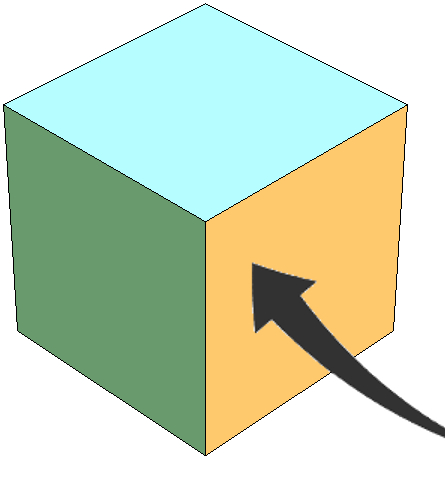 , the crop volume mouse mode

• origin  x,y,z
Place the grid origin at coordinates x,y,z (numbers separated by commas but not spaces).

• originIndex  i,j,k
Place the coordinate origin (0,0,0) at grid indices i,j,k (numbers separated by commas but not spaces). Fractional and negative values are allowed, as the origin is not required to coincide with a grid point or even to fall within the grid.

• voxelSize  S | Sx,Sy,Sz
Voxel size indicates the scale of the data set, the spacing of points in units of distance. If a single number is supplied, it is used in all three directions; if three numbers are supplied (separated by commas but not spaces), they are used in the X, Y, and Z directions, respectively. The grid is anchored at the coordinate origin (originIndex remains unchanged).

• symmetry  sym-type
Assign the specified symmetry to the volume data set. This information is retained in files saved in Chimera map format and can be used by other commands such as molmap, sym, and fitmap. For automatic symmetry detection and assignment, see the command measure symmetry. Most sym-type options have additional sub-options or parameters:

• symmetry of model #N – use “biological assembly” information from an atomic model (currently only read from PDB format, not mmCIF) or the symmetry assignment of another volume model
  • Example: #4
• cage model (from Cage Builder) polygon symmetry #N,pM or #N,pnM – place copies at equivalent positions relative to each M-sided polygon in the cage model with ID number N. The pM form places one copy per M-sided polygon, whereas pnM places M copies per M-sided polygon using CM symmetry about the center of the M-sided polygon nearest the original copy.
  • Examples: #2,p6 or #2,pn5
• cyclic symmetry Cn around axis and center
  • Example: C3
• dihedral symmetry Dn around axis and center
  • Example: d7
• tetrahedral symmetry T[,orientation] around center
  • Example: t,z3
  where orientation can be:
  • 222 (default) – with two-fold symmetry axes along the X, Y, and Z axes, a three-fold along axis (1,1,1)
  • z3 – a three-fold symmetry axis along Z, another three-fold axis in the YZ plane such that rotation about the X axis by ~110° is a symmetry operation (EMAN convention)
• octahedral symmetry O around center
• icosahedral symmetry I[,orientation] around center
  • Example: i,n25
  where orientation can be:
  • 222 (default) – with two-fold symmetry axes along the X, Y, and Z axes
  • 2n5 – with two-fold symmetry along X and 5-fold along Z
  • n25 – with two-fold symmetry along Y and 5-fold along Z
  • 2n3 – with two-fold symmetry along X and 3-fold along Z
  • 222r – same as 222 except rotated 90° about Z
  • 2n5r – same as 2n5 except rotated 180° about Y
  • n25r – same as n25 except rotated 180° about X
  • 2n3r – same as 2n3 except rotated 180° about Y
• helical symmetry H,rise,angle,n[,offset] around axis and center
  • Example: h,43.5,21,6,-2
  where rise is the translation along the axis per subunit, angle is the rotation in degrees per subunit, and n is how many copies total (including the original) the resulting segment of infinite helix should contain. The integer offset (default 0) allows extending the helix in both directions. The example above would give n = 6 copies total, with two copies in the negative axis direction, one at the identity position, and three in the positive axis direction.
• translational symmetry shift,n,distance along axis – or – shift,n,x,y,z
  • Example: shift,3,26.7
  where n is how many copies total (including the original) the result should contain. The translation can be expressed as a distance along the axis or as a vector x,y,z in the reference coordinate system.
• the product of symmetry groups, each specified as described above and separated by * to indicate multiplying each symmetry matrix of one group with each symmetry matrix of another; can be generalized to multiple symmetry groups (not just two)
  • Example: c2*h,42,21,9,-4

• axis  vector-spec
Specify axis of symmetry vector (default z).

• center  point-spec
Specify center of symmetry point in physical coordinates (default 0,0,0). This option is overridden by centerIndex.

• centerIndex [ i | i,j,k ]
Specify center of symmetry in grid coordinates, given as a single value or three values separated by commas only. Grid indices start at zero. Fractional and negative values can be used. If a single value is given, it is used as the grid coordinate along all three axes. This option overrides center.

• coordinateSystem  model-spec
Specify a reference coordinate system for interpreting specifications of axis and center of symmetry.

• dumpHeader  true | false
Whether to write the file header contents (if any) of a map read from MRC or CCP4 format to the Log.

[back to top: volume]

Planes Options     (Usage: volume  model-spec  options)

• planes  axis[,start[,end[,increment[,depth]]]]
Sequentially display slabs depth planes thick along the specified data axis (x,y, or z) starting from index start and repositioning the slab by increment grid units per frame until the index at the next frame would exceed end. The indices refer to the first displayed plane along the axis. If only the axis is given, a single plane at the center of the current display region will be shown. If no end is supplied, only a single slab will be shown. The default increment and depth are both 1. Only planes that are multiples of the step size will be shown, and the depth refers to the number of planes shown rather than a grid index range. Although an increment smaller than the step size can be specified, at each frame the grid index will be rounded down to a multiple of the step size, resulting in the same plane being displayed in more than one frame. To avoid this, change the step size to 1 beforehand or specify start, end and increment values consistent with the current step size. The start, end, increment, and depth parameters can be floating-point numbers. For example, an increment of 0.25 with step size 1 will show each plane for 4 frames. See also: topography, , the move planes mouse mode , volume tile

Pausing the cursor over a single-plane display shows the voxel indices and data value in a pop-up balloon.

• expandSinglePlane  true | false
Expand a single-plane display along its perpendicular axis to the full thickness of the data. This option does not apply to orthogonal planes.

• orthoplanes  xyz | xy | yz | xz | off [ positionPlanes  i,j,k ]
Display planes perpendicular to the X, Y, and/or Z data axes within the current display region. If only a single plane is shown beforehand, it will be expanded to define the region. The positionPlanes option specifies plane locations along the axes by integer grid indices (default 0,0,0 or the lowest indices in the current display region). Orthogonal planes automatically use the image display style, opaque color mode, and an outline, although these can be overriden with the corresponding command options. Turning orthogonal planes off restores the auto8 color mode. See also: , the move planes mouse mode

• boxFaces  true | false
Show data values on the six box faces of the current display region. If only a single plane is shown beforehand, it will be expanded to define the region. Box-face planes automatically use the image display style, opaque color mode, and an outline, although these can be overriden with the corresponding command options. Turning box-face planes off restores the auto8 color mode.

[back to top: volume]

Surface and Mesh Display Options     (Usage: volume  model-spec  options)

The surface and mesh display styles both depict isosurfaces.

• surfaceSmoothing  true | false
Whether to smooth surface and mesh displays. Smoothing entails moving each vertex a specified fraction of the way toward the average position of its neighbors a specified number of times.

• smoothingIterations  N
How many iterations of smoothing to perform (default 2) when surfaceSmoothing is set to true. Each vertex is moved once per iteration.

• smoothingFactor  f
How far to move each vertex when surfaceSmoothing is set to true. In each iteration, each vertex is moved a fraction f (ranging from 0.0 to 1.0, default 0.3) of the way toward the average position of the vertices connected to it by triangle edges.

• subdivideSurface  true | false
Whether to subdivide each triangle in surface and mesh displays into four smaller triangles a specified number of times. A triangle is subdivided by connecting the midpoints of its edges. Subdivision can help to produce smoother surfaces when combined with the surfaceSmoothing option.

• subdivisionLevels  j
How many times to subdivide triangles when subdivideSurface is set to true. The number of triangles is increased by a factor of 4^j, where j is a positive integer (default 1).

• smoothLines  true | false
Turn on anti-aliasing to smooth lines in mesh displays. Mesh lines with transparency > 0.0 can only be smoothed when dimTransparency is true. A side effect of OpenGL anti-aliasing is that dense meshes look brighter from some viewpoints and darker from others, depending on the order in which the lines were drawn.

• squareMesh  true | false
Display only a subset of the lines in the triangular mesh. Lines in the square mesh show the intersection of the XY, YZ, and XZ grid planes with the contour surface.

• dimTransparency  true | false
Decrease the brightness of surface and mesh displays as their transparency is increased. When dimming is on, OpenGL (alpha,1–alpha) blending is used instead of (1,1–alpha) blending.

• meshLighting  true | false
Make the inside of a mesh-enclosed volume dimmer than the outside by varying the brightness according to the angle between each surface point normal and the line of sight. Brightness is maximal when the outward-facing normal is parallel to the line of sight and pointing at the user (see more on the definition of “outward” under flipNormals). When this option is off, the brightness does not vary with the angle between the normal and the line of sight. See also: material

• twoSidedLighting  true | false
Light both sides of surface displays. Otherwise, only the outside of a surface-enclosed volume will be lit (see more on the definition of “outside” under flipNormals). The brightness of each lit side varies according to the angle between a surface point normal and the line of sight; brightness is maximal when the normal is parallel to the line of sight.

• flipNormals  true | false
Affects surface displays when twoSidedLighting is set to false, mesh displays when meshLighting is set to true. When flipNormals is true, the side toward larger or more positive values is treated as the outside for negative thresholds and the side toward smaller or more negative values is treated as the outside for positive thresholds (appropriate for data in which the sign is meaningful, such as electrostatic potential). When flipNormals is false, the side toward smaller or more negative data values is always treated as the outside.

• capFaces  true | false
Cover the faces of the volume data box where high values would be exposed.

[back to top: volume]

Image Display Options     (Usage: volume  model-spec  options)

The image display style shows data as a semitransparent solid. The following options apply to this style.

• imageMode  mode
The mode can be any of the following:

• orthoplanes – orthoplanes
• box faces – box faces of the current display region
• tilted slab – a slab of the data at any angle relative to the data axes (can also be enabled with tiltedSlab true), with additional options:
  • tiltedSlabAxis  vector-spec – slab orientation expressed as a vector perpendicular to the slab
  • tiltedSlabOffset d – position along the axis, where d is the inner product of the vector p (a point on the slab) and the axis vector: d = (p,axis)
  • tiltedSlabPlaneCount N – slab thickness in number of planes
  • tiltedSlabSpacing s – plane spacing in Å
• full region – return to showing the full contents of the current display region after showing orthoplanes, box faces, or a tilted slab

Typically, the graphical interface would be used rather than commands: Map icons or the Volume Viewer display-style menu would be used to switch the image mode, and in the tilted slab mode, slab orientation would be adjusted with the rotate slab mouse mode , slab offset with either the rotate slab button + Shift or the move planes mouse mode , and slab thickness with the crop volume mouse mode . In virtual reality, the rotate slab mode can both rotate the tilted slab and translate it along its axis. The initial tilted slab is perpendicular to the line of sight, with center at the center of the current display region, thickness set to 1/5 of the planes in the current display region along X, Y, or Z (whichever is least), and spacing equal to the smallest of the X, Y, or Z spacing of the data grid.

• backingColor  color-spec 
Specify a backing color (default none) for rendering when the image mode is full region or tilted slab. A dark backing color such as black may improve data visibility when the background color is white or some other light color.

• colorMode  cmode
Specify color pixel format (OpenGL texture format). Possible values of cmode combine a string describing the types of information:

• rgba – multiple colors and transparency
• rgb – multiple colors, opaque
• la – luminance (single color) and transparency
• l – luminance (single color), opaque
• auto – set the mode based on the current display

... with a number of bits: 4, 8, 12, 16. For example, the default cmode is auto8. See also: graphics quality

• projectionMode  pmode
Specify projection mode to adjust the memory-efficiency of display. Possible values of pmode:

• auto (default except for DICOM )
• 2d-x
• 2d-y
• 2d-z
• 2d-xyz
• 3d (default for DICOM )
• rays – raycasting

Displaying just the planes perpendicular to one data axis (2d-x, 2d-y, or 2d-z) uses less memory than automatically switching to those along the data axis most perpendicular to the screen at a given time (2d-xyz). The auto setting uses 2d-z for volumes with a high aspect ratio (second-longest box dimension at least 4 times the shortest box dimension), otherwise 3d. The 3d mode avoids jumps in brightness during rotation by continuously generating planes perpendicular to the line of sight, spaced according to the planeSpacing option. Raycasting may improve the appearance (for example, to be more similar to that in dedicated medical-image rendering programs) with some increase in computational demands; the rayStep option controls the number of samples along each ray. Raycasting is not intended for viewing planes/orthoplanes or tilted slabs. See also:

• planeSpacing  spacing
What spacing to use with projectionMode 3d, with possible values:

• min (default) – smallest spacing of the data along X, Y, or Z
• max – largest spacing of the data along X, Y, or Z
• mean – mean of the data spacing along X, Y, and Z
• d – a specific distance in physical units of length

• rayStep  fraction
With projectionMode rays, how far apart to space samples along each ray, expressed as a fraction of the ray length (default 0.01). In other words, 1/fraction is the number of samples along each ray.

• dimTransparentVoxels  true | false
If true (default), scale voxel brightness in image displays by a factor of (1–transparency). If false, increasing the transparency makes a volume appear brighter because less light is blocked. The appearance option also adjusts this setting.

• colormapExtendRight  true | false
The thresholds and connecting lines on each histogram define a transfer function that maps data values to colors and intensities. This option specifies whether the function should be extended horizontally from the rightmost threshold to the maximum data value at the far right of the histogram (default true).

• colormapExtendLeft  true | false
The thresholds and connecting lines on each histogram define a transfer function that maps data values to colors and intensities. This option specifies whether the function should be extended horizontally from the leftmost threshold to the minimum data value at the far left of the histogram (default false).

• colormapOnGpu  true | false
Whether the mapping of volume data values to colors should be done on the GPU (if true) or CPU (if false). The default is true for DICOM, otherwise false. Colormapping with the GPU is faster but done every time the scene is drawn, whereas colormapping with the CPU is only done when the colors change. Colormapping with the GPU may also give a better, less noisy appearance because the data values rather than the resulting color values are interpolated.

• colormapSize  N
Specify the size of the color lookup table (default 2048) for colormapping on the GPU (any data type) or on the CPU with floating-point data. For color mapping on the CPU with 8-bit or 16-bit map data, this value is ignored and sizes 256 and 65536 are used instead so that each data value has its own color.

• fullRegionOnGpu  true | false
Whether to keep the data (or colors, if colormapOnGpu is false) for the full volume region on the GPU to allow fast cropping. The default is true for DICOM, otherwise false. It is best to use this option with colormapOnGpu true; otherwise, updating colors for the full region even when only a smaller region is shown may slow performance significantly.

• blendOnGpu  true | false
Whether image-display color blending of multichannel data should be done on the GPU (if true) or CPU (if false; default). Color blending on the GPU is about an order of magnitude faster.

• maximumIntensityProjection  true | false
At each pixel, display the the most intense color value underlying the pixel along the line of sight. The maximum intensities of the red, green, and blue color components are determined separately, and transparency is ignored. This option can be useful for enhancing detail. Unphysical effects can result, but are usually not very noticeable; examples include the disappearance of a dim spot when it passes in front of a brighter spot and the simulation of a single spot when the maximal values of different color components under the same pixel actually come from different spots.

• btCorrection  true | false
Correct brightness and transparency for the viewing angle. Without this correction, the apparent brightness and transparency of image displays (in projection modes other than 3d) will depend on the viewing angle relative to the data axes. For a cube-shaped volume with equal resolution in the X, Y, and Z dimensions, the brightness drops and the transparency increases by a factor of 3^1/2 (approximately 1.7) as the viewing angle is changed from along any axis to along the cube diagonal. The brightness correction remedies this, but doubles rendering time.

• minimalTextureMemory  true | false
Reuse a single 2D texture for image displays (in projection modes other than 3d) instead of allocating separate textures for every plane of the data. This is useful for viewing large data sets that would otherwise fail to display, but can degrade interactive response.

• linearInterpolation  true | false
Linearly interpolate brightness and transparency between voxels in image displays. Turning interpolation off may yield a pixelated appearance but speed up rendering, depending on the graphics hardware.

• appearance  preset-name
Apply an image appearance preset, a previously defined collection of display settings for maps in the image display style. The preset-name should be enclosed in quotation marks if it contains any spaces. See also: ChimeraX DICOM Reference

Available presets include:

• approximate implementations of settings from the Horos and MRIcroGL programs for medical image visualization and analysis:
  • Horos “3D presets” as listed on github (with dimTransparentVoxels false); these are generally intended for rendering thicker slabs rather than single planes
    
    
  • MRIcroGL color lookup tables (CLUTs): CT_Bones, CT_Kidneys, CT_Liver, CT_Lungs, CT_Muscles, CT_Skin, CT_Soft_Tissue, CT_Vessels, and CT_w_Contrast (with dimTransparentVoxels true and transparency 0.05)
  
  
• ChimeraX built-in presets, also available via Medical Image icons:
  •  airways – blue airways
  •  chest – yellow bones, blue airways, some other tissues in pink
  •  brain – yellow for fat and similar soft tissue, white of increasing intensity for brain on up to bone, blue for compact bone
  •  initial – (re)set to the threshold levels and colors chosen automatically for the data when first shown as image, with dimTransparentVoxels true, generally useful for planes or thin slabs. DICOM data are initially shown as image with thresholds: (–1000,0),(300,0.9),(3000,1).
  
  
• custom presets defined with the nameAppearance option

• nameAppearance  preset-name
• nameForget  preset-name
Save (or forget a previously saved) preset for the image display style, including threshold levels and colors, brightness, transparency, and dimTransparentVoxels settings. The nameAppearance option requires specifying a volume model currently shown in the image style so that its settings can be saved, for example:

volume #1 nameAppearance brain100

Such user-defined presets are stored in the preferences for later application with the appearance option. Built-in presets (including those available via icons, see above) can be redefined, but “forgetting” their custom definitions with nameForget will revert to their built-in definitions.

[back to top: volume]

Setting Defaults for New Maps

Usage: volume defaultvalues [ saveSettings  true | false ] [ reset  true | false ]  map-options

The volume defaultvalues commmand allows users to set default options for subsequently opened maps. Maps that are already open, if any, will not be affected. The defaults apply only within the current ChimeraX session unless saveSettings true is used to save them as user preferences. Using reset true returns all of the relevant settings to their factory defaults. Giving volume defaultvalues without arguments reports the current set of user defaults in the Log. See also: initial map display

The possible map-options are numerous and described in detail in their respective sections:

• General Display Options:
  • initialColors
  • showOutlineBox
  • OutlineBoxRgb
• Sampling and Size Options
  • limitVoxelCount
  • voxelLimit
  • showOnOpen
  • voxelLimitForOpen
  • showPlane
  • voxelLimitForPlane
  • dataCacheSize
• Planes
  • positionPlanes
• Surface and Mesh Display (all options in section)
  • surfaceSmoothing
  • smoothingIterations
  • smoothingFactor
  • subdivideSurface
  • subdivisionLevels
  • smoothLines
  • squareMesh
  • dimTransparency
  • meshLighting
  • twoSidedLighting
  • flipNormals
  • capFaces
• Image Display
  • backingColor
  • colorMode
  • projectionMode
  • planeSpacing
  • dimTransparentVoxels
  • colormapExtendRight
  • colormapExtendLeft
  • colormapOnGpu
  • colormapSize
  • fullRegionOnGpu
  • blendOnGpu
  • maximumIntensityProjection
  • btCorrection
  • minimalTextureMemory
  • linearInterpolation
  • tiltedSlabAxis, tiltedSlabOffset, tiltedSlabPlaneCount, tiltedSlabSpacing

[back to top: volume]

Volume Operations (Map Editing)

A volume operation edits density maps or other volume data to create a new volume data set. The original map is undisplayed and the new map is displayed with the same threshold and color as the original. Several of these operations are also implemented as graphical tools (e.g., Map Filter). See also: Map Coordinates, Segment Map, surface operations, smoothlines, topography, Map icons

Examples:

volume add #2-25 onGrid #1
vol add #1,2,5 onGrid #5 inPlace true
vol add #1,2 boundingGrid false
vol gaussian #3 sd 5
vol subtract #2 #4 modelId #5
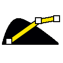
vol unbend #1 path #2 yaxis z xsize 200 ysize 200

Several operations are available:

• volume add – add two or more maps
• volume bin – reduce data size by averaging over cells of multiple grid points
• volume boxes – extract cubic regions centered on markers or atoms
• volume copy – copy map or subregion
• volume cover – extend map to cover specified atoms or box
• volume erase – erase (zero or set to other constant) map values inside or outside a defined sphere
• volume falloff – smooth the boundaries of masked density
• volume flatten – scale values to flatten map baseline
• volume flip – reverse data planes along a specified axis
• volume fourier – Fourier transform
• volume gaussian – Gaussian smoothing
• volume laplacian – Laplacian filtering
• volume localCorrelation – calculate map-map correlation over a sliding box
• volume mask – mask a map to a surface; see also volume onesmask
• volume maximum – take the maximum values pointwise from two or more maps
• volume median – set each value to the median of values in a surrounding box
• volume minimum – take the minimum values pointwise from two or more maps
• volume morph – morph (interpolate) between two or more maps
• volume multiply – multiply values in two or more maps
• volume new – create empty (zero-valued) map; see also volume onesmask
• volume ~octant – erase positive octant
• volume octant – erase all but the positive octant
• volume onesmask – create map with values of 1 bounded by a surface
• volume permuteAxes – permute axes
• volume resample – resample a map on a different grid
• volume ridges – skeletonize; emphasize ridges or filaments in the density
• volume scale – scale, shift, normalize, and/or cast to a different data value type
• volume sharpen – B-factor sharpening
• volume splitbyzone – split map by zones previously colored with color zone
• volume subtract – subtract another map from the first
• volume threshold – reassign values that are below a specified minimum and/or above a specified maximum
• volume tile – make a single-plane volume from tiled slices of another volume
• volume unbend – unbend a map near a path formed by markers/links or atoms/bonds
• volume unroll – unroll a cylindrical slab into a flat slab
• volume unzone – show the full extent of a map previously limited to a zone with volume zone
• volume zone – limit the display to a zone around specified atoms, or make a new map with values of zero at grid points within or beyond the zone

Add two or more maps to create a new map. Option keywords are the same as for volume minimum, volume maximum, and volume multiply:

The scaleFactors keyword indicates multipliers for each map (default 1.0), specified by either:

• as many values as input maps, separated by commas but not spaces
• the word fromlevels, meaning to scale each map by 1/level, where level is the highest surface threshold (contour level) of that map; each map must have a surface with nonzero highest threshold level

The new map can be created on the grid of another map specified with onGrid, where gridmap is a model number preceded by #. If gridmap is not specified, it defaults to the first in volume-spec (the first of the maps being added). The input maps are resampled on the grid by trilinear interpolation, and the resulting values summed for each grid point. Note resampling causes some loss in resolution (details...). Further options related to gridmap:

• spacing – use a finer or coarser grid spacing; if a single distance value is supplied, it is used along all three axes; if three values are supplied (separated by commas but not spaces), they are used along the X, Y, and Z axes, respectively. Using a finer grid reduces the loss of resolution from resampling (details...).
• boundingGrid – whether to adjust (extend or shrink) the grid of gridmap to bound the input maps (default true when adding maps without specifying a gridmap, otherwise false)
• gridStep – whether to use the full resolution of gridmap (step size 1, default) or a specified subsample (step size > 1). Step sizes must be integers. If a single number is supplied, it is used along all three axes; if three numbers are supplied (separated by commas but not spaces), they are used along the X, Y, and Z axes, respectively.
• gridSubregion – whether to use the full extents of gridmap (all, default) or subregion specified by: grid indices i1–i2 along the X axis, j1–j2 along the Y axis, and k1–k2 along the Z axis. Grid indices must be integers separated by commas but not spaces. Grid indices start at zero.

The value-type defaults to the current type of the onGrid map (if any), otherwise the first in volume-spec, and can be 8-, 16-, or 32-bit signed integer (int8, int16, or int32), 8-, 16-, or 32-bit unsigned integer (uint8, uint16, or uint32), or 32- or 64-bit floating-point (float32 or float64).

The hideMaps option indicates whether to hide the input maps (default true).

If the new map is large, for example a whole tomogram, the command may fail for lack of memory. The whole new map must fit in memory.

Average over cells of multiple grid points in the original map to produce a smaller map. Supplying a single integer N (default 2) indicates partitioning the map into bins of NxNxN grid points and averaging the N³ values per bin to produce a new map with 1/N as many points in each dimension. Cells with different numbers of grid points in each dimension can be specified by supplying three integers N_x,N_y,N_z separated by commas only.

For each marker or atom in atom-spec, extract a surrounding cube of data. If useMarkerSize is false (default), the edge length of each cube must be specified in physical units of length with size or in grid units with isize. If useMarkerSize is true, the diameter of its central marker or atom is used as the edge length or added to the size value if also given (default d = 0.0). The isize option facilitates getting the same-sized cubes for each marker, except where a marker is too close to the edge of the density map to obtain a cube of the requested size. If size is used instead, rounding may yield edges that differ slightly in grid dimensions. Marker/atom size can be changed with the size command.

Copy all or a subregion of a map to a new map. The value-type defaults to the same as the input map and can be 8-, 16-, or 32-bit signed integer (int8, int16, or int32), 8-, 16-, or 32-bit unsigned integer (uint8, uint16, or uint32), or 32- or 64-bit floating-point (float32 or float64). The other options are described below. See also: combine, mcopy

Extend a map to cover specified atoms or to fill a rectangular box, using map symmetries and periodicity. The output dimensions can be specified as:

• atomBox spanning the specified atoms plus any extra pad in each dimension (d is in units of physical distance, default 5.0)
• box or just individual dimensions x, y, and/or z in the X,Y,Z coordinate system of the input map
• fbox or just individual dimensions fx etc. in fractional coordinates where 0.0-1.0 spans each dimension of the input map
• ibox or just individual dimensions ix etc. in grid indices of the input map. The input map's grid indices start at 0.

Unspecified dimensions will be kept the same as the input map. The output grid will have the same spacing and alignment as the grid of the input map. The cellSize option specifies unit cell dimensions in grid units along the X, Y, and Z axes. The default unit cell dimensions correspond to the full size of the map, or for CCP4 and MRC maps, are taken from the header. The useSymmetry option indicates whether to use any symmetries associated with the map (default true); if false, only unit cell periodicity will be used. Map symmetries are read from the CCP4 or MRC file header, or can be assigned manually with the symmetry option of volume. or automatically with measure symmetry.

Values from symmetry copies are determined by trilinear interpolation (with potential loss in resolution, see details). Where symmetries and periodicity give multiple copies of the input map overlapping a grid point, the average value will be assigned. The maximum difference between values from different copies at a grid point will be reported in the Log. If there are grid points not covered by symmetry or unit cell periodicity, a message will be sent to the Log, and the points will be assigned values of 0.0. To ensure complete coverage by symmetry copies, the asymmetric unit of the map should extend far enough that its symmetry copies overlap by a non-zero amount. For example, if the unit cell is 100 grid points wide and there is two-fold symmetry along the X axis, the asymmetric unit would need to contain at least 52 grid points along the X axis. If it contains only 50, the two symmetric copies will not overlap, and values in the space between the copies cannnot be determined because the current code cannot interpolate between different copies of the map. If it contains 51, the two copies will have a single plane of grid points in common. Although that would be sufficient with exact arithmetic, the copies still might not overlap given the rounding errors inherent in computer calculations.

Erase (set values to zero, unless a different new-value is given with the value option) the displayed map at points within a sphere of the specified center and radius, or if outside is true, erase outside the sphere instead. Only a single map should be displayed. If the map was read from a file, a copy will be generated automatically and displayed (and the original hidden) so that erasures apply only to the copy. Center coordinates are interpreted in the scene coordinate system unless the coordinateSystem of model N is specified. See Map Eraser for placing the sphere interactively.

Smooth the boundaries of a masked map by replacing the value at each grid point outside the boundary with the average of the values of its six nearest neighbors, for M iterations (default 10). All grid points with values of zero before the first iteration are taken to be outside the boundary, thus assigned a new value at each iteration. Thanks to Greg Pintilie for the initial implementation.

If the method is multiply (default), scale data values by factor (a*i + b*j + c*k + d) where i,j,k are the grid indices and a,b,c,d are calculated to zero out the first moments of the resulting map (make its mass balance at the center of the grid). If the method is divide, data values are divided by the factor (a*i + b*j + c*k + d), which is a least-squares fit to the map data values. For both methods, the a,b,c,d coefficients are scaled to make (a*i + b*j +c*k + d) equal to 1 at the center of the map. If a fitregion is specified, the calculation of the a,b,c,d coefficients uses only the data values in the specified region, while the scaling operation applies to the entire map or the part specified with subregion. The fitregion can be the full extents of the data (all, default) or a subregion specified by grid indices i1–i2 along the X axis, j1–j2 along the Y axis, and k1–k2 along the Z axis. Grid indices must be integers separated by commas but not spaces.

Reverse data planes along a specified axis (default z, reversing the order of the Z planes).

Calculate the 3D Fourier transform. If phase is false (default), generate a magnitude map; if phase is true, generate a map of phase values (–π to π) instead.

Perform Gaussian filtering, where σ is one standard deviation of the 3D Gaussian function in the physical distance units of the map, typically Å (default 1.0). Different standard deviations along X,Y,Z can be specified as three values separated by commas only. Gaussian filtering attenuates high frequencies to smooth the map; however, the opposite behavior (amplifying the high frequencies to sharpen the map) can be specified with invert true. Sharpening with σ values smaller than the pixel size is most useful; larger values overemphasize high frequencies, in effect amplifying noise.

Alternatively, the width of the Gaussian can be specified with bfactor B instead of sDev σ, where B = 8π²σ². See also: volume sharpen

The value-type defaults to the current type and can be 8-, 16-, or 32-bit signed integer (int8, int16, or int32), 8-, 16-, or 32-bit unsigned integer (uint8, uint16, or uint32), or 32- or 64-bit floating-point (float32 or float64).

Gaussian smoothing improves the ratio of signal to noise but reduces resolution. It is fastest for data sizes that are powers of 2, and can be very slow when insufficient memory is available. It may be helpful to limit the input to just a subsample or subregion of the original data. Although it uses a fast Fourier transform calculation method, it does not use map periodicity. Values outside the map boundaries are treated as zero. See also:

Perform Laplacian filtering. The Laplacian operation is a sum of second derivatives. Laplacian filtering is useful for edge detection but amplifies noise, so it may be necessary to perform smoothing such as Gaussian filtering beforehand. Finite differences v(i-1)-2*v(i)+v(i+1) along each axis are used, and voxels at the edge of the box are set to zero.

Calculate the correlation between two maps over a sliding box of NxNxN grid points, generating a new map by assigning the correlation value to the box center. The sliding box is based on the grid of the first map, and N = 5 grid units by default. If the grids of the two input maps do not coincide, the values of the second map will be interpolated (with potential loss in resolution, see details). The subtractMean option specifies whether to subtract the mean of the values in the window from each value in the window before calculating the correlation. The output map will be N–1 smaller in each dimension than the first map.

Mask a map to a surface (details...). The fullMap option indicates making the new map dimensions the same as the full dimensions of the original map, even if only a subregion is being displayed; otherwise (default), the new map will be made as small as possible to enclose the surface. The pad option allows extracting a larger or smaller region by moving the surface a positive or negative distance (in the distance units of the data, typically Å or nm) along surface normals before creating the masked volume. However, if the resulting surface intersects itself, the masked volume will not include the intersection. For larger-region extraction, this problem can be avoided by instead using the extend option to move the surface outward by N voxels before creating the masked volume. In other words, extend includes grid points that are within N grid units (along the grid X, Y, and Z axes) of the original surface.

The slab option allows instead extracting a slab of data around a surface layer. Two additional surfaces, displaced as specified from the existing surface and joined at their edges (if any), are computed but not displayed. Data for voxels between the computed surfaces are retained. If a single value (width) is supplied, the two computed surfaces are offset along the normals of the original surface by ±½(width). Alternatively, two values separated by a comma but no spaces can be used to specify the offsets of the two surfaces independently. Positive or negative values can be used.

The invertMask option allows getting the opposite result (spatial complement of values and zeros) of what would otherwise be obtained.

The region between surface layers is computed along the projection axis (a vector specified in the map coordinate system, default y). The axis direction matters when the surface has holes. The sandwich option specifies including only volume voxels between paired surface layers; if false, the volume projected along the axis beyond a single surface layer will also be included. When intersecting or nested surfaces are involved, the fillOverlap option indicates retaining the union of the values from masking to each surface separately. For example, if the surface(s) include two concentric spheres, fillOverlap true will return values for all grid points within the larger sphere, whereas fillOverlap false will return values for only those points in the shell between the two surfaces.

The related command volume onesmask creates a new map with values of 1 bounded by a surface. See also: volume multiply, shape, surface invertShown, segmentation, segger exportmask, Segment Map

Set each value to the maximum at that point in two or more input maps. See volume add for descriptions of the options.

Smooth the data by setting each value to the median of the values in a box centered at that point. Values at points for which the surrounding box extends outside the data are simply set to zero. Box dimensions are specified in grid units with binSize and must be odd integers. Supplying a single integer N (default 3) indicates a box size of NxNxN grid points. Boxes with different numbers of grid points in each dimension can be specified by supplying three integers N_x,N_y,N_z separated by commas only. The iterations option indicates how many cycles of smoothing to perform (default 1).

Set each value to the minimum at that point in two or more input maps. See volume add for descriptions of the options.

Morph between two or more maps. The morph can be played back with the slider graphical interface. For a reasonable result, the input maps should have the same grids: dimensions, spacing, and numbers of points. Note volume resample can be used to make a copy of one map that has the same grid as another. A morphing fraction of 0.0 corresponds to the first map and a fraction of 1.0 corresponds to the last, with intermediate maps evenly spaced within that range. There is smooth interpolation between each adjacent pair of maps.

The morph display will proceed from start-fraction (default 0.0) in steps of increment (default 0.04) for N frames (default 25). By default (playDirection 1), the initial direction of play is from low to high fractions. If the number of frames and step increment are more than needed to reach the playRange bounds (default is the entire range: 0.0,1.0), the morph display will “bounce” back and forth. The scaleFactors keyword specifies a multiplier for each map (details...). The constantVolume option specifies adjusting the threshold (contour level) automatically to keep the enclosed volume constant. The addMode option specifies treating the second map as a delta to be added to the first instead of linearly interpolating between the two. It is not recommended for inputs of >2 maps. The hideOriginalMaps option specifies hiding the input maps. The interpolateColors option only applies when the maps have the same number of thresholds (contour levels for surface/mesh display, coloring control nodes for image display).

The slider option (default true) shows a graphical interface for volume morph playback. The slider can be dragged or a frame number entered directly. The interface also includes a play/pause button, a    value to increase for slower playback, and a button for recording a movie (). Sequential integers are added to the movie filename (movie1.mp4, movie2.mp4, ...) so that repeated recordings will not overwrite the previous ones, and the save location can be set with the snapshot command. The movie will start at the current slider position, so to include the whole morph, place the slider at the far left before clicking the record button.

The Loop Playback setting in the slider context menu controls whether interactive playback should continue until explicitly paused (initially on). The Bounce Playback setting in the slider context menu is only available when Loop Playback is on, and controls whether looping wraps from end to beginning so that playback is only in the forward direction (initial setting, Bounce Playback off) or alternates between forward and backward (Bounce Playback on). These loop/bounce settings apply only to interactive viewing, not recording a movie with the button mentioned above.

The morph is created as a new map (volume) model. However, if the modelId of an existing map is given, the existing map model will be reused instead of a new one being added. In other words, to “replay” a morph without losing its coloring, zoning, or transparency settings:

1. use volume morph an initial time to create the morph model
2. apply coloring, zoning, etc. as desired to that model
3. use volume morph again, but this time specifying the modelId of the existing model so that its properties will be retained during playback

See also: vseries, morph, making movies

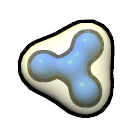
Multiply the values pointwise in two or more maps. This is used to apply a mask (values 0,1) to a map. See volume add for descriptions of the options. See also: volume mask

Create an “empty” zero-valued map named map-name (default new) with the specified size (number of grid points along each axis, default 100), gridSpacing in physical distance units (default 1.0 along each axis), origin coordinates (default 0.0,0.0,0.0), and cellAngles (default 90,90,90°; a single value can be supplied if α = β = γ). Grid size and spacing can each be given as a single value to apply to all three axes or as three values separated by commas only. If map-name includes spaces, it must be enclosed in quotation marks. The value-type defaults to float32 and can be 8-, 16-, or 32-bit signed integer (int8, int16, or int32), 8-, 16-, or 32-bit unsigned integer (uint8, uint16, or uint32), or 32- or 64-bit floating-point (float32 or float64). See also: volume onesmask

Erase values inside the positive octant (all grid points with X,Y,Z coordinates greater than the center). The center can be specified in physical units (such as Å) with center or in grid units with iCenter, where grid indices start at zero. The default is the center of the volume data box. The coordinates should be separated by commas but not spaces, and the values can be fractional. iCenter overrides center if both are given. The values in the erased regions will be set to value (default 0). A different value may improve contour surface appearance; for example, large negative values produce flatter surfaces where an octant has been cut away from a map of positive values.

Erase values outside the positive octant. Options are as described for volume ~octant above.

Create a map with values of 1 bounded by a surface (details...). The onGrid option allows creating the new map on the grid of another map specified by model number, gridmap, using either its full extents (fullMap true, default) or the smallest needed to enclose the surface (fullMap false).

Alternatively (if onGrid is not used):

• the border option indicates how far out from the bounding surface in all six directions (±X, ±Y, ±Z) to place the edge of the output map
• the spacing option gives the grid spacing for the output map in physical units of length, typically Å (default is 1% of the maximum of the X, Y, and Z dimensions of the bounding surfaces). If a single number is supplied, it is used in all three directions; if three numbers are supplied (separated by commas but not spaces), they are used in the X, Y, and Z directions, respectively.

The value-type defaults to the current type of the onGrid map (if any), otherwise int8; the choices are 8-, 16-, or 32-bit signed integer (int8, int16, or int32), 8-, 16-, or 32-bit unsigned integer (uint8, uint16, or uint32), or 32- or 64-bit floating-point (float32 or float64). The remaining options are the same as described for volume mask. See also: volume new, shape

Permute grid axes to the specified axis-order, which can be any of the 6 ordered combinations of x, y, and z. The original order is xyz.

Skeletonize map(s) by tracing along high-density grid points to identify ridges or filamentous structures in the density. At each grid point, the value is compared to the values of all the points in the surrounding 3x3x3 box, and the count of how many directions (up to 13) along which the value is a local maximum is assigned as that point's value in the new map. The level keyword indicates a minimum value in the original map below which to automatically set the new value to 0, essentially ignoring those points in the skeletonization. The default minimum is the lowest display threshold (contour level) in the original map. Viewing the new skeleton map with a threshold of 6-10 highlights ridgelike features in the original map.

Resample values to a different grid using trilinear interpolation. Resampling causes some loss in resolution (details...). One or both of the following options must be supplied:

• use the grid of another map specified with onGrid, where gridmap is a model number preceded by #
• use a finer or coarser spacing of points on the grid; if a single distance value is supplied, it is used along all three axes; if three values are supplied (separated by commas but not spaces), they are used along the X, Y, and Z axes, respectively. Using a finer grid reduces the loss of resolution from resampling (details...).

The other arguments are as described above for volume add.

Shift values by adding a constant (default 0.0), scale values by a multiplicative factor f (default 1.0), and/or cast them to a different data value type. When values are both shifted and scaled, the shift is applied first. Two normalization options calculate a scaling factor from the data:

• rms – scale values to make new-rms = ((∑x²)/N)^½ where x is each value and N is the total number of values
• sd – first shift values so that the mean is 0.0, then scale values to make new-std-dev = ((∑x²)/N)^½

If a factor f is also specified, it is applied last. The value-type defaults to the current type and can be 8-, 16-, or 32-bit signed integer (int8, int16, or int32), 8-, 16-, or 32-bit unsigned integer uint8, uint16, or uint32), or 32- or 64-bit floating-point (float32 or float64).

See also: rmsLevel, sdLevel options of volume, measure mapstats

Perform B-factor sharpening. This amplifies high frequencies by dividing by a Gaussian in frequency space. The width of the Gaussian can be specified with bfactor B, which is in units of Ų and relates to the real-space standard deviation σ of the function according to B = 8π²σ². Alternatively, the width can be specified with sDev σ (default 1.0 Å). Different standard deviations along X,Y,Z can be specified as three values separated by commas only. Sharpening amplifies high frequencies; however, the opposite behavior (damping the high frequencies to smooth the map) can be specified with invert true. Sharpening with σ values smaller than the pixel size is most useful; larger values overemphasize high frequencies, in effect amplifying noise.

All other options are the same as described for volume gaussian above. See also:

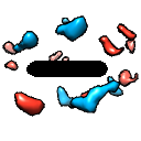
Split a map by zones previously colored with color zone. A new map is created for each distinct color and for the “uncolored” zone (any parts of the original map not within a color zone). Values outside the respective zones are set to zero. The new data sets are created as submodels of a new model named by appending “split” to the name of the original map. See also: Segment Map

Subtract the values of othermap from map, both specified by model number preceded by #. The scaleFactors option specifies multipliers for the two maps, either:

• f1 and f2 for map and othermap, respectively, separated by a comma but not a space
• the word fromlevels, meaning to scale each map by 1/level, where level is the highest surface threshold (contour level) of that map; each map must have a surface with nonzero highest threshold level

Alternatively to using scaleFactors, if minRms is true, othermap will be scaled automatically to minimize the root-mean-square sum of the resulting (subtracted) values at grid points within the lowest contour of othermap.

The new map can be created on the grid of another map specified with onGrid, where gridmap is a model number preceded by #. If gridmap is not specified, it defaults to map. The input maps are resampled on the grid by trilinear interpolation, and the resulting values subtracted for each grid point. Note resampling causes some loss in resolution (details...).

The remaining arguments are as described above for volume add, except that boundingGrid always defaults to false. When subtraction from an unsigned-integer map could give negative numbers, the valueType option should be used to specify a signed data type for the result.

See also: , the subtractMaps option of fitmap

Replace all values that are below a mininum value (min) with newmin (default equal to min), and/or replace all values that are above a maximum value (max) with newmax (default equal to max).

Create a single-plane volume by tiling slices of a specified volume perpendicular to the specified axis (default z). The spacing of slices in grid units (default 1) is given with the pstep keyword. The trim keyword indicates each slice should be trimmed on all four edges by i grid units (default 0). The slices are arranged into a single plane with number of rows r and number of columns c. If neither the number of rows nor the number of columns is supplied, they are computed to produce as near a square tiling as possible. If one or the other is supplied, the remaining parameter is adjusted to accommodate the total number of slices. The fillOrder setting (default ulh) specifies the tiling pattern, including the starting corner, the tiling direction (horizontal or vertical), and whether to reverse the order of slices. The first two characters specify the corner for the first tile, the first character being u for upper or l for lower and the second being l for left or r for right. These directions are defined with the specified axis pointing at the viewer and the remaining two axes pointing up and right. The third character is h for horizontal tiling or v for vertical tiling. The optional fourth character r indicates that the order of the slices should be reversed. The resulting volume data set has the same origin and orientation of axes as the original volume, and grid size 1 along the specified axis.

Unbend a map near a path formed by markers/links or (equivalently) atoms/bonds. The path-spec should be an atom-spec that specifies a single chain of atoms (markers) connected by bonds (links). The path will be mapped to the Z axis of the result. The yaxis setting indicates which axis in the existing volume should be mapped to the Y axis of the result, and can be given as x, y (default), z or any of the other standard vector specifications. The gridSpacing s is the separation between grid points in the new map (default is the minimum spacing along the three axes of the input map). The xsize xs and ysize ys are the X and Y dimensions of the new map in physical units, typically Å (default 10 times the new grid spacing). A cubic spline is placed through the path points and the input volume is interpolated on planes perpendicular to the splined path.

Unroll a hollow cylindrical section of the map into a flat slab. Cylinder axis (default z) and center (default 0,0,0) coordinates are interpreted in the coordinate system of the input map, unless another reference model is specified with coordinateSystem. The dimensions of the cylindrical slab are given in physical units of length, typically Å: length d (default is the map extent parallel to the cylinder axis) and inner and outer radii r1 and r2 (defaults are 90% of the smallest radius and 110% of the largest radius of the displayed isosurface, respectively, given the cylinder center and axis direction). The flattening is done by interpolating values from the original map on a cylindrical grid of points, then unwrapping the cylindrical grid into a rectangular grid. The cylinder radial direction becomes the X-axis of the new map, circumference the Y-axis, and cylinder axis direction the Z-axis. The gridSpacing s is the requested separation of grid points along each axis in the new map (default is the minimum spacing along the three axes of the input map). The actual spacing may be slightly different because the dimensions of the new map may not be an exact multiple of the requested value; the number of grid divisions along each axis is chosen to give spacing as close as possible to the requested value without being smaller.

Show the full extent of a map that was previously limited to a zone using volume zone with option newMap false.

If newMap is false (default), limit the surface display to a zone within range r (default 3.0 Å) of any atom in atom-spec, and if minimalBounds is true, restrict the current display region of the map to the smallest rectangular box containing the zoned surface. The corresponding Map icon uses a range value six times the grid spacing of the map. The full extent of the map can be restored with volume unzone. The invert option is not available with newMap false.

If newMap is true, create a new map in which the values of grid points beyond the zone are set to zero, or if invert is true, with values within the zone set to zero. If minimalBounds is also true, make the resulting map as small as possible while enclosing the zone; otherwise, the dimensions will be the same as for the input map. If bondPointSpacing is specified, use points spaced s Å apart along bonds in addition to the atoms to define the zone. See also: surface zone, color zone, zone, the zone mouse mode

New-Map Options

modelId  N
Open the new data set as model number N (an integer, optionally preceded by #). The default is the lowest unused number.

step  N | Nx,Ny,Nz
Whether to use the full resolution of the data (step size 1, default) or a specified subsample (step size > 1). Step sizes must be integers. A step size of 1 indicates all data points, 2 indicates every other data point, 3 every third point, etc. If a single number is supplied, it is used along all three axes; if three numbers are supplied (separated by commas but not spaces), they are used along the X, Y, and Z axes, respectively.

subregion  i1,j1,k1,i2,j2,k2 | all
Whether to use the full extents of the data (all, default) or a subregion specified by grid indices i1–i2 along the X axis, j1–j2 along the Y axis, and k1–k2 along the Z axis. Grid indices must be integers separated by commas but not spaces. Grid indices start at zero.

inPlace true | false
Whether to overwrite the existing data set instead of creating a new one. *Not all volume operations accept this option.* Regardless of this setting, the existing data will only be overwritten if it was created in ChimeraX (for example, with a previous volume operation) rather than read from a file. In the case of map addition, the model to overwrite is the gridmap (the model whose grid will be used for the result).

[back to top: volume]

Notes

Resampling and loss of resolution. There is some loss of resolution with resampling a map on a different grid with trilinear interpolation. The effect is similar to smoothing. The amount of reduction in resolution depends on the initial resolution, the initial and final grid spacing, the “bumpiness” of the data, and the shift between the grids. For example, starting with a 6-Å resolution map with 2-Å spacing from molmap and resampling on a grid (with the same spacing) shifted by 1 Å reduced resolution to approximately 7.7 Å. Starting with a 6-Å resolution map with 1-Å spacing and resampling on a grid shifted by 0.5 Å reduced resolution to approximately 6.4 Å. Resampling to a finer grid can be specified with the spacing option of the command.

Transfer function. For image displays, the thresholds and connecting lines on the histogram define a transfer function that maps data values to colors and intensities. For each voxel, the data value is compared to the thresholds on the histogram. The colors and intensities of the closest threshold at a lower data value (to the left) and the closest threshold at a higher data value (to the right) are linearly interpolated. Color is defined by red, green, blue and opacity components. The intensity at a threshold is further scaled by its vertical position, where 0 is the bottom of the histogram and 1 is the top. Unless the function is extended horizontally to the maximum and/or minimum value, voxels with data values greater than the rightmost threshold or less than the leftmost threshold are colorless and completely transparent. Rendering time does not depend on the positions of the thresholds, but increases with greater numbers of thresholds.

Image transparency details. For image displays, the transfer function maps a voxel's data value to a vertical position (ranging from 0 to 1) on the histogram. A lower position indicates more transparency:

T_histogram = 1 – vertical position

T_pixel = T_histogram^(1/p)

Byte order. Different computers store the bytes of a single numeric value in different orders. PowerPC processors use one order (called big-endian), while Intel/AMD x86 family processors use the opposite order (called little-endian). If a binary data file is created on one machine and read on another having the opposite byte order, byte-swapping is required to get the correct numeric values. The DSN6 file reader assumes that the file was written in big-endian byte order. DSN6 files can be read on big- or little-endian machines. All of the other file readers detect file byte order and machine byte order, then perform byte-swapping if necessary.

Fourier transform. Only the magnitudes of the complex Fourier components are included in the new data set; the phases are discarded and the constant component is set to zero. The box containing the Fourier transform (with axes in units of reciprocal space) is centered on the original data and scaled to have the same total volume. Some properties of the original data are evident from the Fourier transform. High-frequency components are near the edges of the box, low-freqency components near the center. Volume data is typically oversampled (voxel size two to three times smaller than the actual data resolution) and this causes the Fourier transform to have nonzero values only in the middle half or third of its bounding box. The missing wedge in electron microscope tomograms can also be seen. Spikes radiating along the principal axes in the Fourier transform are caused by nonperiodicity of the original data.

Mask algorithm. The masked volume is computed by finding where lines parallel to the projection axis intersect the surface(s). For a given line, the volume data between the 1st and 2nd, 3rd and 4th, 5th and 6th, ... points of intersection are included in the masked volume, while those between the 2nd and 3rd, 4th and 5th, ... are excluded (unless there are intersecting or nested surfaces and fillOverlap is set to true). The calculation uses a set of parallel lines that pass through points on a rectangular grid perpendicular to the projection axis. If the projection is along a data axis (data X, Y, or Z), the lines will pass through the grid points of the data; otherwise, lines along the projection axis with spacing equal to the minimum grid plane spacing of the data will be used. For each volume voxel, the intersections of the closest grid line are used to determine inclusion in the masked volume. If there is an odd number of intersections, then points beyond the final one are not included in the masked volume unless the sandwich option is set to false. In the new data set, values outside the masked region are set to zero and those inside are set to the original volume values (for volume mask) or 1 (for volume onesmask). The grid points of the calculated volume align exactly with those of the original volume, if any.